Quick Check: From Last Time
Before we move, let's try those questions from the last session on Wednesday, July 08, 2026, about word embeddings.
❓ Question 1
In your own words: what is a word embedding, and why is it useful for a language model?
❓ Question 2
We measured how alike two words are using cosine similarity. What does a value close to 0 tell us about the two words?
❓ Question 3 (multiple choice)
Word embeddings place similar words close together in vector space. Which pair would you expect to have the highest cosine similarity?
A) “king” and “queen”
B) “king” and “pizza”
C) “king” and “airplane”
D) “king” and “banana”
(No right or wrong — these just warm up our intuition. A full recap is on the next slide.)
Want to refer back? Last session's deck (on GitHub Pages): → Embeddings deep-dive
How Meaning Works: Embeddings → Similarity
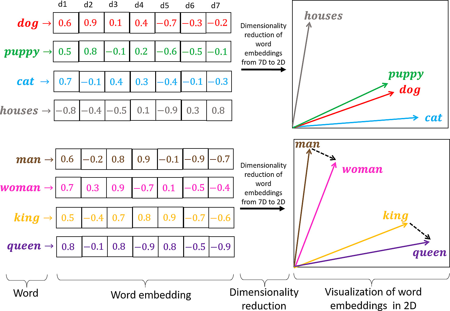
A full t-SNE example from scratch. We see how a word's vector captures meaning, how the dot product combines two vectors, and how cosine similarity measures how alike their meanings are.
Dataset — 5 words with 3D embeddings
| Word | Vector (3D) | What it represents |
|---|---|---|
| dog | [6, 9, 1] | Strong positive in dim 1 & 2 |
| puppy | [5, 8, -1] | Very similar to dog, slight difference |
| man | [6, -2, 8] | Strong in dim 1 & 3, slightly negative dim 2 |
| woman | [7, 3, 9] | Strong in all dimensions |
| tree | [-7, -8, -3] | All negative (opposite direction to animals) |
Visual intuition: dog & puppy point in nearly the same direction · man & woman point in similar directions · tree points in the opposite direction from dog.
Step 1 — Cosine similarity formula
cos(A,B) = (A·B) / (|A| × |B|)
A·B = dot product (multiply matching numbers, add them). |A| = length (Euclidean norm) of A.
Step 2 — Vector Norms
| Word | Calculation | |vector| |
|---|---|---|
| dog | √(36+81+1)=√118 | √118 ≈ 10.86 |
| puppy | √(25+64+1)=√90 | √90 ≈ 9.49 |
| man | √(36+4+64)=√104 | √104 ≈ 10.20 |
| woman | √(49+9+81)=√139 | √139 ≈ 11.79 |
| tree | √(49+64+9)=√122 | √122 ≈ 11.05 |
Step 3 — Dot products
dog·puppy = 30+72-1 = 101 | dog·man = 36-18+8 = 26 | dog·woman = 42+27+9 = 78
dog·tree = -42-72-3 = -117 | puppy·man = 30-16-8 = 6 | puppy·woman = 35+24-9 = 50
puppy·tree = -35-64+3 = -96 | man·woman = 42-6+72 = 108 | man·tree = -42+16-24 = -50 | woman·tree = -49-24-27 = -100
Step 4 — Cosine similarities
| Pair | Calculation | cos |
|---|---|---|
| dog–puppy | 101 / (10.86×9.49) | 0.98 |
| dog–man | 26 / (10.86×10.20) | 0.23 |
| dog–woman | 78 / (10.86×11.79) | 0.61 |
| dog–tree | -117 / (10.86×11.05) | -0.98 |
| puppy–man | 6 / (9.49×10.20) | 0.06 |
| puppy–woman | 50 / (9.49×11.79) | 0.45 |
| puppy–tree | -96 / (9.49×11.05) | -0.92 |
| man–woman | 108 / (10.20×11.79) | 0.90 |
| man–tree | -50 / (10.20×11.05) | -0.44 |
| woman–tree | -100 / (11.79×11.05) | -0.77 |
Interpretation: dog–puppy 0.98 (almost identical) · man–woman 0.90 (both humans) · dog–tree −0.98 (opposite meaning) · dog–woman 0.61 (both living things) · puppy–man 0.06 (barely related).
Your Turn: Calculate Similarity Yourself
Use cos(A,B) = (A·B) / (|A|×|B|). For each pair: (1) dot product, (2) each vector's length, (3) divide. Then check against the matrix on the previous page.
Problem 1 — dog vs tree
dog = [6, 9, 1]
tree = [-7, -8, -3]
Dot product = ____ |dog| = ____ |tree| = ____
cosine = ____ Similar or opposite?
Problem 2 — dog vs man
dog = [6, 9, 1]
man = [6, -2, 8]
Dot product = ____ |dog| = ____ |man| = ____
cosine = ____ Weakly or strongly related?
Problem 3 — man vs woman
man = [6, -2, 8]
woman = [7, 3, 9]
Dot product = ____ |man| = ____ |woman| = ____
cosine = ____ What does this tell us?
Bonus: Pick your own pair from the dataset, or invent two 3D vectors and compare answers with a neighbour.
What We'll Build in 2 Hours
1. BPE From Scratch
Build the same algorithm that powers GPT-4 & Gemma — in pure Python. Learn exactly how text becomes numbers.
2. Sliding Window
Turn raw text into thousands of "context → target" flashcards. This is how every language model learns.
3. Tiny Transformer
Build a miniature neural network that predicts the next word. Watch the loss go down as it learns.
4. Text Generation
Give it a prompt like "Jide was" and watch it autocomplete a story. Real AI, running live.
No prior ML experience needed. Just Python basics and curiosity.
One-Time Setup
Open the Colab Notebook or your local Python environment. Run these two blocks:
# Import everything we need
import re, math
from collections import defaultdict, Counter
import numpy as np
import matplotlib.pyplot as plt
import torch, torch.nn as nn
from torch.nn import functional as F
import tiktoken

# Check for GPU
device = 'cuda' if torch.cuda.is_available() else 'cpu'
print(f"Running on: {device.upper()}")💻 Local users
pip install torch numpy matplotlib tiktoken in your virtual env.
How Do We Turn Text Into Numbers?
Computers don't understand words. They understand numbers. Tokenization is the bridge.
Three Ways to Split Text
Word-level
["Cassava","is","a","crop"]
Simple but fails on new words. Need huge vocabulary (500K+ words).
Character-level
["C","a","s","s","a","v","a"," ","i","s",...]
Handles any word but makes very long sequences — slow training.
Subword (BPE)
["Cass","ava","is","a","crop"]
Best of both worlds. Common words = 1 token. Rare words = split into pieces.
BPE (Byte-Pair Encoding) is what GPT-4, Gemma, LLaMA, and Claude all use.
How BPE Works (Simple Version)
Imagine you're a toddler learning to read. You start with letters, then notice some pairs appear together a lot.
Step 1
Split every word into individual letters + a word-end marker </w>
Example: "crop" → "c r o p </w>"
Step 2
Count every adjacent pair. Find the most frequent one.
("c","a"): 2 times, ("a","</w>"): 9 times ...
Step 3
Merge the winner into a new single token everywhere.
"c a" → "ca" (now treated as one unit)
Step 4
Repeat until you reach your target vocabulary size.
50 merges → 80 tokens. 1000 merges → 1000+ tokens.
BPE in Action — Example
Tracing BPE on a tiny corpus: "sunny rainy sunny". Watch letters merge into subwords, step by step. (</w> marks the end of a word.)
| Iteration | Merge | Resulting Tokens |
|---|---|---|
| Start | — | s u n n y </w> r a i n y </w> s u n n y </w> |
| 1 | n + y → ny | s u n ny </w> r a i ny </w> s u n ny </w> |
| 2 | s + u → su | su n ny </w> r a i ny </w> su n ny </w> |
| 3 | su + n → sun | sun ny </w> r a i ny </w> sun ny </w> |
| 4 | sun + ny → sunny | sunny </w> r a i ny </w> sunny </w> |
| 5 | sunny + </w> → sunny</w> | sunny</w> r a i ny </w> sunny</w> |
Each step merges the most frequent neighbour pair. In just 5 merges, "sunny" becomes a single token — so the model treats it as one meaningful unit instead of six separate letters.
BPE in 4 Functions
We only need 4 small functions to build BPE from scratch.
get_vocab()
Break text into words → split into characters → add </w>
get_stats()
Count how often every pair of symbols appears together.
merge_vocab()
Replace the most frequent pair with a new merged token.
bpe_train()
Loop: count → merge → repeat until target vocab size.
def get_vocab(corpus):
    vocab = {}
    for word in corpus.lower().split():
        tokenized = " ".join(list(word)) + " </w>"
        vocab[tokenized] = vocab.get(tokenized, 0) + 1
    return vocab

def get_stats(vocab):
    pairs = defaultdict(int)
    for word, freq in vocab.items():
        symbols = word.split()
        for i in range(len(symbols) - 1):
            pairs[(symbols[i], symbols[i+1])] += freq
    return pairs

def merge_vocab(pair, vocab):
    a, b = pair
    merged = a + b.replace("</w>", "")
    pattern = " ".join([a, b])
    new_vocab = {}
    for word, freq in vocab.items():
        new_vocab[word.replace(pattern, merged)] = freq
return new_vocabLet's Train It!
We'll feed BPE sentences about African farming and watch it learn.
CORPUS = "Cassava is a major food crop in Nigeria and across sub-Saharan Africa. Farmers in Kenya grow maize beans and sweet potatoes. The cocoa industry in Ghana and Ivory Coast produces most of the world's chocolate. Climate change affects rainfall patterns across East Africa. Drought resistant crops like millet and sorghum are important for food security. Smallholder farmers use sustainable farming practices to improve crop yields."

# Train to 50 total tokens (starts from ~30 letters)
merges, final_vocab, _ = bpe_train(CORPUS, vocab_size=50)

# Sample output you'll see:
Merge 1: 'a' + '</w>'  →  "a</w>"
Merge 5: 't' + 'h'    →  "th"
Merge 10: 'in' + 'g'   →  "ing"
Then we tokenize a new sentence:
test = "Farmers grow cassava in Nigeria"
tokens = tokenize_bpe(test, merges)
print(tokens)  # → ['Farm', 'ers', 'grow', 'cass', 'ava', 'in', 'Nig', 'eri', 'a']
Notice how "cassava" splits into cass + ava — the algorithm learned that "cass" and "ava" are useful subwords!
Switch to a Production Tokenizer
Our custom BPE works, but it only has 50 tokens. Real LLMs use 100,000+ tokens. Let's use tiktoken — the tokenizer behind GPT-4.
# Tiktoken has ~100K tokens trained on billions of pages
enc = tiktoken.get_encoding("cl100k_base")

# Our tiny story for training
raw_text = """Jide was hungry so she went looking for food. She checked the market, but it was closed. Then, she found a small cafe and ordered some rice and water. She was very happy to finally eat!"""

# Encode: text → numbers
data = torch.tensor(enc.encode(raw_text), dtype=torch.long)

print(f"Characters: {len(raw_text)} → Tokens: {len(data)}")
# Output: "Characters: 188 → Tokens: 43"

# Decode a token back to prove it works
print(enc.decode([data[0].item()]))  # → "Jide"
43 tokens to represent 188 characters. That's the power of a good tokenizer — it compresses text efficiently.
Embeddings: Words as Vectors
A number alone (token ID) has no meaning — "397" and "401" don't tell us the words are related. Embeddings fix this by mapping each token to a vector of numbers where similar words live close together.
Token ID → Vector
Each token gets its own embedding — a list of, say, 32 numbers. Think of it as a coordinate in meaning-space.
Similar → Nearby
"cat" and "dog" have similar vectors (both pets). "king" is close to "queen" but far from "apple". The model learns these relationships.
Learned During Training
Embeddings start as random noise. As the model trains, it pushes/pulls words closer or farther apart to capture meaning.
Embedding for "king" → [0.23, -1.45, 0.67, ..., 0.12]  (32 numbers)
Embedding for "queen" → [0.25, -1.40, 0.62, ..., 0.15]  (very similar!)
Embedding for "apple" → [-0.98, 2.10, -0.33, ..., 0.88]  (very different)
Last session you explored embeddings in depth — t-SNE maps and cosine similarity. Today we put them to work: those same vectors become the model's memory, learned live as it trains.
Creating Training Data: The Sliding Window
A language model's only job: predict the next token. We create flashcards: "Given these tokens, what comes next?"
block_size = 8  # How many tokens the model sees at once
batch_size = 4  # How many examples we process together

def get_batch():
    ix = torch.randint(len(data) - block_size, (batch_size,))
    x = torch.stack([data[i:i+block_size] for i in ix])  # Context
    y = torch.stack([data[i+1:i+block_size+1] for i in ix])  # Target
return x.to(device), y.to(device)The model sees 8 tokens at a time and must predict token #9. We make thousands of these from our tiny story.
The Tiny Brain: Our SLM Architecture
A miniature version of what powers ChatGPT. Three parts:
1. Token Embedding
Each token ID → a vector of 32 numbers. Similar words get similar vectors.
nn.Embedding(vocab_size, n_embd=32)
2. Position Embedding
Each position (1st, 2nd, 3rd...) → a vector. Helps the model know word order.
nn.Embedding(block_size, n_embd)
3. Linear Head
Predicts which token comes next. Like a "what's the most likely next word?" machine.
nn.Linear(n_embd, vocab_size)
class TinySLM(nn.Module):
    def __init__(self, vocab_size, n_embd):
        super().__init__()
        self.token_embedding_table = nn.Embedding(vocab_size, n_embd)
        self.position_embedding_table = nn.Embedding(block_size, n_embd)
        self.lm_head = nn.Linear(n_embd, vocab_size)

    def forward(self, idx, targets=None):
        B, T = idx.shape
        tok_emb = self.token_embedding_table(idx)
        pos_emb = self.position_embedding_table(
            torch.arange(T, device=device))
        x = tok_emb + pos_emb
        logits = self.lm_head(x)
        if targets is None:
            return logits, None
        B, T, C = logits.shape
        loss = F.cross_entropy(logits.view(B*T, C), targets.view(B*T))
        return logits, loss
The two embedding tables are the heart of the model — they store the meaning of every word, exactly the vectors you explored last session. Training is just the model learning better embeddings so it can predict what comes next.
Total: ~6.5 million parameters. Tiny by today's standards (GPT-4 has trillions), but enough to learn patterns!
Training: Becoming Less Wrong
A fresh model guesses randomly. Training fixes that — one tiny adjustment at a time.
1. Forward Pass
Feed context, get prediction, calculate loss. Loss = "how wrong are we?" (lower is better)
2. Backward Pass
Use loss.backward() to calculate the gradient — the direction to nudge each weight.
3. Update Weights
optimizer.step() applies the nudges. The model becomes slightly less wrong.
optimizer = torch.optim.AdamW(model.parameters(), lr=1e-3)

for step in range(600):
    xb, yb = get_batch()                # Grab a batch
    logits, loss = model(xb, yb)         # Forward pass
    optimizer.zero_grad(set_to_none=True)
    loss.backward()                      # Backward pass
    optimizer.step()                     # Update weights
    if step % 100 == 0:
        print(f"Step {step}: Loss = {loss.item():.4f}")
Watch the loss go from ~10 (random guessing) down to ~1.5 (learning patterns).
Let It Speak!
After training, our tiny model can generate text. We give it a starting word and ask: "What comes next?"
def generate(self, idx, max_new_tokens, temperature=1.0):
    for _ in range(max_new_tokens):
        idx_cond = idx[:, -block_size:]         # Only use last 8 tokens
        logits, _ = self(idx_cond)               # Predict
        logits = logits[:, -1, :] / temperature  # Scale by temperature
        probs = F.softmax(logits, dim=-1)        # Convert to probabilities
        idx_next = torch.multinomial(probs, 1)   # Sample
        idx = torch.cat((idx, idx_next), dim=1)  # Append
    return idx
Temperature trick: Lower = more focused/repetitive, Higher = more creative/risky. Try temperature=0.8!
Making Our Model Smarter
Our first model was tiny (32-dim embeddings, 8-token context, 600 steps). Let's level up.
↑ block_size: 8 → 32
Wider context window = the model sees more of the story before predicting. More coherent text.
↑ n_embd: 32 → 64
Richer token representations. Each word gets a more detailed vector. Better pattern capture.
↑ Steps: 600 → 5000
More training = more chances to learn. Each pass refines the weights a little more.
Result: A model that generates much more coherent text. Try it in Colab — change these 3 numbers and watch the difference!
Scale the recipe further: The same architecture at a larger size reaches 12,937,781 parameters — more capacity means more patterns it can capture. (Our BiggerSLM uses ~6.5M; bigger still = smarter still.)
What You Learned Today
1. BPE builds vocabulary by merging frequent pairs
Start with characters, merge the most common pair, repeat. The merge order reveals language patterns.
2. Vocab size controls efficiency
Smaller vocab = more tokens per word (handles rare words). Larger vocab = fewer tokens (faster, but bigger model).
3. Sliding window creates training data
Every language model learns by predicting the next token. The sliding window turns raw text into context→target flashcards.
4. Even tiny models can learn patterns
With only ~6.5M parameters and a 4-sentence story, our model learned to generate coherent text. That's the magic of neural networks.
💡 The big idea: Every word's meaning lives in its embedding — the same vectors you explored last session. When we train this little model, we are really just learning better embeddings so it can predict the next word. That's the whole magic of language models!
Thank You!
Questions? Let's discuss.
TRI AI Saturdays · Cohort 10 · In partnership with Google DeepMind